


When computing and AI pioneer Alan Turing (1912–1954) first proposed his “Imitation Game” in 1950 as a test of artificial intelligence, it was framed in terms of gender recognition:
I propose to consider the question, ‘Can machines think?’ This should begin with definitions of the meaning of the terms ‘machine’ and ‘think’. […] Instead of attempting such a definition I shall replace the question by another, which is closely related to it and is expressed in relatively unambiguous words.
The new form of the problem can be described in terms of a game which we call the ‘imitation game’. It is played with three people, a man (A), a woman (B), and an interrogator (C) who may be of either sex. The interrogator stays in a room apart from the other two. The object of the game for the interrogator is to determine which of the other two is the man and which is the woman. […]
We now ask the question, ‘What will happen when a machine takes the part of A in this game?’ Will the interrogator decide wrongly as often when the game is played like this as he does when the game is played between a man and a woman? These questions replace our original, ‘Can machines think?’ 1

What we now call the Turing Test takes a gender-neutral form; it involves a human judge trying to determine whether the entity at the other end of an online chat is another human or a machine. It’s telling, though, that in his original formulation, Turing’s challenge subverted what he regarded as the epitome of human judgment: making a gender determination without relying on physical cues.
There’s something very meta about a closeted gay mathematician in postwar Britain proposing to test whether a machine can pass for a man trying to pass for a woman. But of course, in the fifties, binary gender (and heterosexuality) were requirements to be recognized as fully human. So, perhaps Turing was being subversive in more than one way.
In her sharp analysis of the Imitation Game paper, literary critic N. Katherine Hayles wrote,
By including gender, Turing implied that renegotiating the boundary between human and machine would involve more than transforming the question of “who can think” into “what can think.” It would also necessarily bring into question other characteristics of the […] subject, for it made the crucial move of distinguishing between the enacted body, present in the flesh on one side of the computer screen, and the represented body […] in an electronic environment. This construction necessarily makes the subject into a cyborg, for the enacted and represented bodies are brought into conjunction through the technology that connects them. […] As you gaze at the flickering signifiers scrolling down the computer screens, no matter what identifications you assign to the embodied entities that you cannot see, you have already become posthuman. 2
Certainly, embodiment matters. On the other hand, when we interact with others socially—whether by text, video, or in the flesh—only parts of our bodies are disclosed, while others are covered up. In this, we differ from our primate kin.
Even naked, though, disclosure is incomplete. Aspects of our embodiment remain opaque to our lovers, and even to ourselves, or it wouldn’t be possible to grow up intersex and not know it. So, it’s not always clear where the boundary lies between a “represented” and “enacted” body.
In an increasingly social and digital world that affords us a growing range of technologies for altering both our bodies and the way we present ourselves to others, it’s also no longer clear which (if either) of these is the “real you.” Having spent the last several chapters delving into the connections between the biology of sex and gender identification, it’s now time to look more carefully at how presentation and behavior relate to identity.
We become Turing’s “interrogator (C)” every time we meet someone new and (despite the increasingly strong injunction never to make assumptions) need to guess which pronoun to use. Practically speaking: How do we do it?
Hopefully you’re convinced by now that gender isn’t something that can be worked out by pure logic, or based on any single variable. It has to be a more holistic (thus necessarily imperfect) judgment, based on the whole “fuse box” of gendered attributes, signals, and behaviors.
Chapter 2 explored handedness from a similarly multidimensional perspective, using optimal linear estimation to correlate dozens of questions about behavior and presentation with personal identity as a left- or right-handed person—or both, or neither. This chapter will apply the same techniques to gender and sexual orientation, allowing us to zoom out from the “trees” of individual responses, which I’ve focused on so far, to see the whole “forest” of presentation.
Recall how a linear estimator for, say, right-handedness produced the optimal set of question weights for calculating a right-handedness score. The same kind of linear estimator can predict the answer to the question “Are you female?” based on answers to 37 of the survey’s behavioral questions. The output is a set of question weights representing the relative importance of each response, ranging from a strong positive correlation (a large positive number), to neutral (near zero), to a strong negative correlation (a large negative number).
Predictably, the question weights for optimally predicting “Are you male?” are virtually identical, but with the positive and negative signs flipped. (Running the same analysis to predict pronoun—exclusively “she” or exclusively “he”—yields nearly identical results.) There are no great surprises in the question weights. Which bathroom someone uses is the single most predictive variable, while long or short hair, manicures, and waxing are more weakly predictive. 3
As with handedness, a linear estimator can also be calculated to predict ambiguous responses to the gender questions—subjects who answer either “yes” to both, or “no” to both of “Are you female?” and “Are you male?”
Now, hair length becomes far more relevant; short hair is the single most correlated question, while long hair is the most anti-correlated. Bathroom use is no longer so significant, though use of the women’s bathroom is somewhat more common than the men’s, and the use of urinals is nearly as uncommon as long hair, suggesting a desire for greater privacy. Other signs of androgyny are evident too, such as negative correlations with gendered names.
Clearly there are people in the excluded middle, but is this middle the exception, or the norm, behaviorally speaking? Is the gender binary still alive and kicking? And are “both or neither” people really a “third gender,” as has sometimes been claimed?
A mathematical technique called Principal Component Analysis, or PCA, can help address these questions. Using PCA involves taking the set of questions above—which are purely about socially visible behavior and presentation, and don’t include “Are you female?” or “Are you male?”—and finding the internal correlations among them.
It works as follows. Let’s define a “component” as a numerical score calculated just as above: a weighted sum of the answers to the 37 yes/no questions about gender presentation. The “first component” of the PCA is the set of question weights yielding the single most informative score that can be calculated, meaning that knowing this score for any individual would do the best possible job of estimating the answers to all 37 questions. 4
In theory, it could be the case that this one number would suffice to fully describe the data. Imagine, for instance, that we were working with a much smaller set of yes/no questions:
Do you use the women’s bathroom?
Do you use the men’s bathroom?
Do you have long hair?
Do you have short hair?
As many case studies in this book show, one can never safely assume that a person’s response to one of these questions will determine the answer to any other one. There are four variables here, with two potential values each, allowing for 2×2×2×2=16 possibilities of varying popularity. But let’s suppose that we were administering this four-question quiz in an imaginary town—call it Stepford, USA—where everyone answers in only one of two equally likely ways: (+1, −1, +1, −1) for Stepford women, and (−1, +1, −1, +1) for Stepford men, where +1 represents “yes” and −1 is “no.” If we were to carry out a PCA, 5 the first principal component would then have weights corresponding to (+1, −1, +1, −1), or equivalently, (−1, +1, −1, +1), or any other fixed multiple of these numbers, like (+0.5, −0.5, +0.5, −0.5); only the proportions of the weights relative to each other matter. For a stereotypical woman’s responses, this first principal component score would then work out to 0.5×1 + (−0.5)×(−1) + 0.5×1 + (−0.5)×(−1) = +2, while the first principal component value for a stereotypical man’s responses would be 0.5×(−1) + (−0.5)×1 + 0.5×(−1) + (−0.5)×1 = −2. This single score, +2 or −2, would tell us how any given respondent answered all four questions.
Or maybe not! Even in Stepford, a woman might eventually decide to get a bob at the hairdresser’s. The occasional man might even grow his hair out. This would cause a second principal component to emerge, with weights (+0.5, −0.5, −0.5, +0.5). As you can check for yourself, this component will be zero for long-haired women or short-haired men, but will produce a +2 for women with bobs, and a −2 for men with long hair. So in this slightly more complex (and slightly more realistic) situation where hair length doesn’t always coincide with the gender norm, the original four questions need to be represented by two numbers, not just one. The first, and most informative, still encodes gender, while the second is nonzero for anyone with gender-atypical hair length.
So that’s Principal Component Analysis. Let’s now leave Stepford and enter the real world, where I’ve recorded valid responses from 9,578 Americans to all 37 gender presentation questions.
The first principal component that emerges looks almost indistinguishable from the gender prediction weights. Maybe this isn’t surprising, but it is meaningful, since neither sex assigned at birth nor gender identity was an input into the analysis. This result tells us that in the real world, most of the behavioral markers of gender co-vary in a way that closely mirrors people’s identification with a gender. In other words, this one “gender score” emerges organically from the data, and describes more of the variation in it than any other single score would.
Next, let’s look at a histogram of everyone’s first principal component score, that is, the sum of their answers multiplied by these weights.
This histogram has two humps; it looks like the gender binary is alive and well after all. Though on closer inspection, this can’t quite be the full story. For a variable to be described as truly binary, it would have to assume only two values, like the +2 and −2 of our Stepford example. Here, there’s a whole range or spectrum of values along the “gender axis,” from roughly −0.015 to +0.015, with no empty regions along that range.
Nonetheless, there are clearly two peaks, with a less-populated valley in between. The curve looks like the profile of a two-humped camel.

Let’s compare this to a histogram of respondents’ heights. Men are on average taller than women, so overall, the distribution of human height also looks like a sum of two superimposed bell curves; however, because the random variations within the male and female distributions are large compared to the difference between them, no noticeable dip exists in between: the 67 inch or so midpoint (5 feet, 7 inches) remains a common height overall. Hence the sum looks more like a one-hump dromedary (or Arabian camel) than its rarer two-hump cousin.
Because height is an easily measured, reasonably clear-cut biological variable while the presentation variables are more squishy and cultural, it’s tempting to assume that clear-cut “rational” categories apply to biology but not to culture. For example, in a 2022 book on sex differences, primatologist Frans de Waal writes,
Differences between the sexes […] show a bimodal distribution (the famous bell curves), which means that they concern averages with overlapping areas between them. For example, men are taller than women, but only in a statistical sense. We all know women who are taller than the average man, and men who are shorter than the average woman. […] Gender is a different issue altogether [… The terms masculine and feminine] refer to social attitudes and tendencies that aren’t easily classified. They often mix so that aspects of both are manifested in a single personality. […] Gender resists division into two neat categories and is best viewed as a spectrum that runs smoothly from feminine to masculine and all sorts of mixtures in between. 6
Reading this passage, one would guess that height ought to look like a two-hump camel, while a behavioral “gender score” ought to look like a one-hump dromedary, with masculine and feminine traits blending into a featureless continuum; but in fact, it’s the other way round. Human bodies are not so strongly sexually dimorphic on average, making the combined height distribution look more unimodal than bimodal—notwithstanding de Waal’s description of how he and his brothers, like their father, “towered head and shoulders” above their mother. 7 (Though in fairness, adding additional physiological variables, such as weight and muscle mass, would pull the distributions farther apart, up to a point.) A gender presentation score based on those squishy cultural markers, though—clothes, grooming, choice of bathrooms—is clearly bimodal.

Still, while the gender presentation histogram is two-humped, those humps do overlap. So the question of whether gender is binary or not lacks a clear answer. The debate is itself a false binary. Many people, in their presentation, appear to fall clearly into one peak or the other, and the very presence of those distinct peaks suggests categories. Being great pattern recognizers and namers of things, humans would make up names for those peaks if they didn’t already exist. 8 However, the peaks aren’t cleanly separated, so those categories can’t account for everyone’s presentation. There are people living in the valley too.
If you’re paying close attention, you may have noticed that I haven’t yet confirmed whether the two humps in the first principal component histogram actually correspond to sex or gender identification. That question, and more, can be answered by visualizing respondents as points in 2D space, with their coordinates given by their first and second principal component scores—something like a God’s eye view of every respondent in a 2D “gender presentation space.” (The approach can easily extend to 3D.) Points can then be colored based on the respondent’s identification as female, male, both, or neither.
The histogram of respondents’ first principal component scores would result from letting all of these points fall onto the horizontal axis and counting them up in bins. It’s easy to see that the overwhelming majority of the right-hand hump would consist of orange dots—people who identify exclusively as female—while the left-hand hump would consist mostly of turquoise dots—people who identify exclusively as male. In 2D, these humps look like fairly well-defined clusters. However, if you look closely, you can spot a few people whose identities wouldn’t be predicted correctly based on how they present. There are orange dots surrounded by turquoise ones, and turquoise dots deep in orange territory. Moreover, a smattering of “both” and “neither” appears across the entire range of presentations (these are drawn with bigger dots for extra clarity, since they’re sparser).
Visualizations like these might explain why the idea of a “third gender,” as a distinct cluster with specific social markers, has never fully taken off in modern Western culture. 9 “Both” and “neither” points are scattered throughout the whole space, including—but by no means limited to—the excluded middle between conventionally masculine and feminine presentations.
This impression can be confirmed by graphing the likelihoods of female, male, or “both or neither” identification as a function of their score using the optimal linear predictors, just as for left-, right-, and ambiguous-handedness in Chapter 2. Female and male predictors mirror each other, and show near-perfect performance at the extreme ends of the scale, with a transition in between where a greater proportion of “both or neither” people tend to fall. However, “both or neither” is never the likeliest option, even at the most ambiguous point in the middle of the scale, where male or female identification is equally likely. Specifically, at that point of “maximum androgyny,” a person is about 40% likely to identify as male, 40% likely to identify as female, and 20% likely to identify as both or neither.
Consistent with this, an optimal linear predictor for “both or neither”-ness doesn’t exhibit anything like the reliability of the predictors for binary gender. Even for a person maxing out this score, the likelihood of identifying as “both or neither” is only 5% or so, with the remaining majority of the probability split roughly evenly (with large error bars) between female and male identification. An ambiguous “femaleness vs. maleness” score implies much higher odds of being “both or neither”—closer to 20%—but only because far fewer binary respondents fall into that excluded middle. Seen another way, just as many “both or neither” people present the way traditionally female or male people do as present in the excluded middle; it’s just that, in that excluded middle, they stand out more clearly against the sparser binary background. So, “both or neither” people can look any which way. Most aren’t especially androgynous in their presentation.
You may wonder how to interpret “Principal component 2,” the vertical axis in the scatter plot. This second component seems relevant to gender identity too, though less straightforwardly. Notice how the clusters tilt slightly: people whose first component is near zero—that is, who are most ambiguous on the horizontal dimension—are more likely to identify as female, and much likelier to identify as “neither,” if their second component is less than zero (toward the bottom), but more likely to identify as male if the second component is greater than zero (toward the top). Hence, while most of the information one might use to guess someone’s gender is in the first component, knowing the second component would allow for a slightly better guess. (The same is true—though barely—for the third component; a case of diminishing returns.)
High values for this second component correlate with living in the city and working in tech, while low values correlate with living in the suburbs and having long hair. What does it all mean? There may be an interesting story here, but interpretation of second-order effects can start to look more like data art than data science. It all falls in the realm of social signaling, though—in the relevant contexts and communities, people take in this kind of subtle information and use it, often subconsciously, when they make inferences about a stranger’s gender. Conversely, we also use an implicit understanding of these patterns when we make decisions about our own presentation (for instance, at the hair salon).
If one were to run a survey including questions about all of the sex-relevant biological, physiological, and anatomical variables discussed in Chapter 11 (on intersexuality), the first principal component of the answers would almost certainly exhibit the same two-hump pattern. Moreover, many of those physiological variables (such as having larger breasts) strongly correlate with behavioral variables (such as wearing a bra), for obvious reasons—though such correlations may be weakening in the disembodied, online world we increasingly inhabit, which has started to look like a giant worldwide Turing Test arena… one which is, incidentally, also full of bots masquerading as people. 10 So, as we all relocate to the internet and (perhaps) gender fades in importance, the two-hump camel pattern might start to look more like the height histogram’s one-hump dromedary. This idea will be explored further in the next chapter.
As long as we can see each other’s real life faces, though, even in a tightly cropped Zoom window, the overlapping but still clearly two-humped pattern of facial sexual dimorphism—the different average shapes of men’s and women’s faces, allowing reliable classification in a majority of cases—will remain obvious. We’ll also continue to make occasional misgendering mistakes, just as if we were to guess at the colors of dots on the survey PCA based on their position alone.
Like the Turing Test, recognizing facial images is a classic problem in machine intelligence. In 1990, Alex “Sandy” Pentland, a computer science professor at MIT and serial entrepreneur, dedicated his lab’s attention to face recognition. They began by using precisely the techniques described above, simply replacing the 37 yes/no survey response values with a few tens of thousands of pixel values. 11 The researchers aligned uniformly posed and lit digital images of volunteers’ faces, then reduced the resolution to something manageable—256×256 monochrome pixels, each represented by a number between 0 (black) and 1 (white). Averaging those images yields a blurry, indistinct “average face.”

Averages can also be made using the faces of people sharing some trait, to generate composite portraits of specific subpopulations. South African artist Mike Mike did this years later in his itinerant photography project The Face of Tomorrow, 12 which digitally superimposed portraits of men and women grouped by age and, somewhat arbitrarily, by geography. By manually aligning the pupils of the eyes and other facial features, he was able to make his composites a lot sharper than those of the Pentland Lab in the 90s. The results are striking, and the faces are beautiful in their way, though also bland, since asymmetries and distinctive features (including anything one might consider a blemish) have been averaged away. “Average skin” looks smooth and featureless. “Average hair” looks like a diffuse fuzzy mass, since one subject’s individual strands of hair won’t match up precisely with those of any other subject.
Though it may not be immediately obvious, these composites are visualizations of exactly the kind of optimal linear estimators I’ve described for handedness or gender. To understand why, consider how you’d go about calculating the optimal gender weights for the four “Stepford survey” questions earlier in this chapter (“Do you use the women’s bathroom?”, “Do you use the men’s bathroom?”, “Do you have long hair?”, and “Do you have short hair?”). The basic recipe is to calculate a conditional average, meaning that the optimal weights for an “Are you female?” estimator are simply the average of the answers of all of the respondents who said “yes” to “Are you female?”
In the same way, the average face of a young female Sydneysider can serve as a “template for femaleness” among young Sydneysiders. Scoring the relative similarity of a young Sydneysider’s face to this template (which can be calculated by summing the products of a subject’s facial pixels with the template pixels) will predict the likelihood that the subject is female. 13
It’s a seductively simple and powerful trick. Given the data to make such templates, what else might one be able to predict based on a facial image?

Victorian polymath Francis Galton (1822–1911), a pioneer in the statistical method of correlation, originally invented the facial compositing technique—long before we had digital computers. Galton was less interested in gender, though, than in law and order. Like his contemporary and fellow traveler, our old friend Cesare Lombroso, Galton sought to turn old-fashioned policing into a modern scientific discipline: criminology.

In that spirit, he set out to visually characterize “criminal types” by superimposing exposures of convicts on the same photographic plate, 14 a procedure much like what Mike Mike did digitally more than a century later. Making observations and establishing correlations: the scientific method! But is there really such a thing as an “average criminal face”?

Although Galton’s idea contained a kernel of mathematical insight, it suffered from many of the same problems in practice as Lombroso’s pseudo-scientific studies of criminality. For starters, superimposing just a handful of exposures can’t yield anything like a real population average. More importantly, though, the selection of people included will determine what the resulting model “predicts”; as a statistician today might say, garbage in, garbage out. If, for instance, the 19th century Irish were economically disadvantaged, hence likelier to turn to crime, and on top of that likelier to be convicted by the British legal system, then the average “criminal face” probably would look Irish. By a feat of circular logic, this “scientific observation” could then be used to justify anti-Irish prejudice: a vicious cycle. This problem isn’t merely hypothetical. Predictive policing systems today have been built on the same flawed logic. 15

With computers, it’s possible to go beyond the averaged faces Galton could approximate using a handful of exposures on a photographic plate (or Mike Mike’s more refined digital composites) and run a full Principal Component Analysis. The equivalent of the “question weights” for each principal component are a set of positive and negative weights on face pixels, each of which, when applied to an individual face image and added up, produces a score. Visualizing the weights, using black for the most negative, white for the most positive, and medium gray for zero, yields ghostly face-like images (so-called “eigenfaces”), which one can think of as systematically tweaking the average face—adding or subtracting hair in one case, making the forehead and cheekbones more or less prominent in another, and so on.


In this way, just as a questionnaire can be reduced to one or two numbers, a face photo also can be reduced to one or a handful of numerical scores. Forty such numbers (corresponding to the first forty principal components) are enough to uniquely identify an individual, and can easily distinguish feminine-looking faces from masculine-looking ones, much as the first PCA component of the survey does. 16 The result: not just a gender prediction model, but a general system for facial recognition. What could possibly go wrong?
To be sure, face recognition has plenty of valuable and benign uses. Our own brains (or most of them) certainly do face recognition, as do the brains of many other smart visual animals; it powers the capacity for individual recognition described in the Introduction. Neither is there anything inherently sinister about a smart camera that detects faces in the viewfinder to keep them in focus, nor a smartphone with a face unlocking feature uniquely keyed to the phone’s owner.
However, early funding for face recognition didn’t come from phone or camera manufacturers, but from the Defense Department, which coordinated a number of institutions to accelerate its development, starting in 1993. Based on his lab’s promising early results, Sandy Pentland was tapped to help lead this effort. The goal was much the same as that of the revolutionary French government’s Comité de Surveillance, established in every municipality during the Reign of Terror: to develop techniques whereby the state could monitor the movements of outsiders, dissidents, and suspect individuals in general. 17
This French bureaucratic term, surveillance, from sur (over) and veiller (to watch), has since entered the English language too. But whereas blanket surveillance of public spaces used to require vast, shadowy networks of informants, digital face recognition allows it to be automated. Today, the authorities’ “view from above” of citizens’ movements in security camera-saturated cities like Beijing or London far outdoes the analog police states of the 18th, 19th, and 20th centuries.
Recently, the technology has gotten a lot better, too. Manhattan-based startup Clearview AI uses “deep learning,” based on large neural networks rather than simpler “linear” methods like PCA, to supply the FBI, Immigration and Customs Enforcement (ICE), the Department of Homeland Security (DHS), Interpol, and many local police departments (as well as various corporate customers) with truly powerful individual face recognition capability. 18 PCA can be thought of as a simple, “single-layer” artificial neural network; hence, in today’s language, a minimal kind of artificial intelligence or AI system. The many stacked layers that give deep learning its name make systems like Clearview’s both much more accurate and much more robust, so that face images don’t need to be aligned, uniformly posed, or consistently lit, as with PCA. Deep learning can work surprisingly well even when faces are partially hidden, made up, or disguised. 19 Trained on billions of face images scraped from the web and social media, Clearview’s system is said to reliably recognize anyone with an online presence from surveillance photos or video. 20
On one hand, such technology can catch child abusers and foil terrorists. On the other, its indiscriminate deployment can put us all under continuous surveillance, not just by nosy neighbors, but by powerful governments that can mobilize the technology for social control, political repression, or even genocide. Even the US, nominally a democracy whose government must abide by the rule of law, has shown itself perfectly willing to conduct illegal mass surveillance on its own citizens. 21
Perhaps even more troubling are applications of face recognition that don’t aim to recognize known individuals, but rather to make inferences about unknown people based on how they look. Some of these systems revive Francis Galton’s long-dormant fantasy of recognizing “criminal types.” In 2016, for instance, two machine learning researchers, Xiaolin Wu and Xi Zhang, put a paper online, Automated Inference on Criminality Using Face Images, 22 claiming that their deep neural net could predict the likelihood that a person was a convicted criminal with nearly 90% accuracy using nothing but a driver’s license-style face photo. Their training and testing data consisted of 730 images of men wanted for or convicted of a range of crimes by provincial and city authorities in China, as well as 1,126 face images of “non-criminals […] acquired from [the] Internet using [a] web spider tool.”
Although one can’t say for sure what their neural net is really picking up on, given the opacity of their data sources, some suggestive clues are offered by the three examples each of “criminals” and “non-criminals” shown in the paper. For one, the “non-criminals” all wear white-collar shirts, while the “criminals” don’t. There may be a racial profiling component in play here too. 23 The main difference, though, is most likely the frowny faces of the “criminals,” and the smiley faces of the “non-criminals.” (This interpretation is also consistent with measurements the authors offer of average differences in facial landmark positions between the two groups.)


That’s right: the “criminals” look meaner, and the “non-criminals” look nicer! But is that a cause, or an effect? We develop biases against “mean-looking” people early in childhood. Even 3- and 4-year-olds can reliably distinguish “nice” from “mean” face images. 24 Physiognomists, too, have long held the perfectly reasonable-sounding position that nice people have nice faces, and mean people have mean faces.
What, exactly, do these stereotypically “nice” and “mean” faces look like? Researchers studying the social perception of faces in recent years 25 have used (you guessed it) Principal Component Analysis to explore not only this question, but how people’s first impressions of faces work in general. In one experiment, a video game-like face renderer produces a wide range of artificial faces based on 50 numerical measurements; experimental participants then describe their impressions of randomly generated faces, or rate them according to some perceived personality trait. PCA can capture most of the variability in people’s first impressions using just a few components, three of which the researchers have named “dominance,” “attractiveness,” and “valence.” The first two are fairly self-explanatory. The third, “valence,” is associated with positive impressions like “trustworthy” and “sociable.”


An optimal linear predictor lets us visualize what a stereotypically “trustworthy” or “untrustworthy” face looks like, as shown here for white males. Notice how the “trustworthy” face has a more smiley expression—and reads as more feminine—while the “untrustworthy” face is more frowny and more masculine. It’s likely no coincidence that the supposedly “criminal” faces in Wu and Zhang’s paper look a lot like the “untrustworthy” face, while the “non-criminal” faces are more like the “trustworthy” face.
Galton’s composites of “criminal types” also look more like the “untrustworthy” face. They resemble “Prendergast, the Murderer,” a mentally disturbed Irish-born newspaper distributor who assassinated five-term Chicago Mayor Carter Harrison, Sr. on October 28th, 1893.

The following year, an iconic courtroom drawing of Patrick Eugene Prendergast with a downturned mouth made it into the Chicago Tribune. The dour mouth, disembodied like that of a homicidal Cheshire cat, was subsequently immortalized in several American books on physiognomy, warning the reader to beware any bearer of such lips. Perhaps this was indeed Prendergast’s resting face, though given the circumstances—summarized by the caption under the newspaper portrait, “TO BE HANGED TODAY”—it’s hard to be sure.

People make instinctive, automatic judgments about character traits like trustworthiness after seeing a face for less than one tenth of a second. 26 Author Malcolm Gladwell wrote effusively about snap judgments like these in his 2005 bestseller, Blink: The Power of Thinking Without Thinking. It does seem that such judgments do a remarkable job of predicting important life outcomes, 27 ranging from political elections to economic transactions to legal decisions.
The question is, are these good judgments? Either answer would be interesting. If they are good judgments, then the physiognomists are right—we really do advertise our essential character traits on our faces. On the other hand, if those judgments are arbitrary, then that they do such a good job of predicting outcomes tells an even more disturbing story: that unwarranted prejudice based on resting facial appearance plays a decisive role in human affairs.
A large body of research favors the latter interpretation. 28 For example: in 2015, Brian Holtz, of Temple University, published the results of a series of experiments 29 in which facial “trustworthiness” was shown to strongly influence experimental participants’ judgment. The participants were asked to decide, after reading a vignette, whether a hypothetical CEO’s actions were fair or unfair. While the judgment varied (as one would hope) depending on how fair or unfair the actions described in the vignette were, it also varied depending on whether the CEO’s face looked “trustworthy” or “untrustworthy” in the profile photo.
In another study, 30 participants played an online investment game with what they believed were real partners, represented by “trustworthy” or “untrustworthy” faces. Participants were more likely to invest in “trustworthy” partners even in the presence of more objective reputational information about the past investment behavior of their partners.
Even more chillingly, another study 31 found that among prisoners convicted of first degree murder, the unlucky defendants with “untrustworthy” faces were disproportionately more likely to be sentenced to death than to life imprisonment. This was also the case for people who were falsely accused and subsequently exonerated.
So, we’re not endowed with some subconscious Blink-like genius for making snap judgments about people’s characters based on how they look. Unfortunately, we make those snap judgments anyway, sometimes to our own detriment: for instance, studies in which the trustworthiness of economic behavior was measured show that relying on face judgments can make our decisions less reliable than if we were making them, literally, blind. 32
The worst consequences, though, fall upon anyone who happens to have an “untrustworthy” face. For example, it seems that they’ll be significantly more likely, all things being equal, to end up convicted of a crime, while a guilty party with a “trustworthy” face is likelier to get away with their misdeeds. In sum, the facial “criminality detector” tells us more about our own pervasive biases than about the subject’s character.
In the Fall of 2017, a year after the “resting criminal face” paper came out, a higher-profile study 33 began making the rounds claiming that sexual orientation could be reliably guessed based on a facial image. The Economist featured the study on the cover of their September 9th magazine; 34 on the other hand, two major LGBTQ+ organizations, The Human Rights Campaign and GLAAD, immediately labeled it “junk science.” 35
Michal Kosinski, who co-authored the study with fellow researcher Yilun Wang, initially expressed surprise, calling the critiques “knee-jerk” reactions. However, he then doubled down with even bolder claims: that similar approaches will soon be able to measure the intelligence, political orientation, and—you guessed it—criminal inclinations of people from their faces alone. 36
Once again, this echoes the old claims of Cesare Lombroso and Richard von Krafft-Ebing: physiognomy, but now dressed in the “new clothes” of AI. However, while Wu and Zhang seemed well outside the mainstream in tech and academia, Kosinski is a faculty member of Stanford’s Graduate School of Business, and the new study was accepted for publication in the respected Journal of Personality and Social Psychology. Much of the ensuing scrutiny focused on ethics, implicitly assuming that the science was valid. As with the previous year’s result, however, there’s reason to believe otherwise.

The authors trained and tested their “sexual orientation detector” using 35,326 images from public profiles on a US dating website. Composite images of the lesbian, gay, and straight men and women in the sample, 37 reminiscent of Galton’s composites, reveal a great deal about the patterns in these images.


According to Wang and Kosinski, the key differences between the composite faces are in their physiognomy, meaning that sexual orientation tends to correlate with a characteristic facial structure. However, you’ll notice right away that some of these differences are more superficial. For example, the “average” straight woman appears to wear eyeshadow, while the “average” lesbian doesn’t. Glasses are clearly visible on the gay man, and to a lesser extent on the lesbian, while they seem absent in the heterosexual composites. Might it be the case that the algorithm’s ability to detect orientation has less to do with facial structure than with grooming, presentation, and lifestyle?
When the study was published, I was already running the Mechanical Turk surveys that would eventually turn into this book, so I teamed up with a couple of colleagues, Margaret Mitchell, then at Google, and Alex Todorov, then faculty at Princeton’s Psychology Department, to run an extra survey that might shed some light on Wang and Kosinski’s findings. 38 In addition to the usual questions about sexual orientation and attraction, we added a few, like “Do you wear eyeshadow?” and “Do you wear glasses?”; “Do you have a beard or mustache?” and “Do you ever use makeup?” were already on there.
These graphs break down responses by sexual orientation, based both on behavior and identity. “Opposite-sex attracted women” are people who answer “yes” to “Are you female?,” “no” to “Are you male?,” and “yes” to “Are you sexually attracted to men?” and “Are you romantically attracted to men?”; a very similar subset of women answer “yes” to “Are you heterosexual or straight?” “Same-sex attracted women” are those who answer “yes” to “Are you sexually attracted to women?” and “Are you romantically attracted to women?” The curves for men follow the same pattern.
It will surprise no one that, at all ages, straight women tend to wear more makeup and eyeshadow than same-sex attracted and (even more so) lesbian-identifying women—although seen another way, the curves also show that these stereotypes are often violated. Even among opposite-sex attracted women, between a third and half don’t wear eyeshadow, while around half of lesbians in their mid-20s do.
That same-sex attracted people of most ages wear glasses significantly more than exclusively opposite-sex attracted people do might be less obvious, but it is so. What should one make of this? A physiognomist might cook up a theory about gay people having worse eyesight.
It’s unlikely, though. Answers to the question “Do you like how you look in glasses?” reveal that wearing glasses is probably more of a fashion statement, with the fashion trend varying by age. The pattern holds both for women and for men, though the trends seem to be at their most variable among gay (and more generally same-sex attracted) men. Perhaps Elton John had something to do with it?
Answers to the question “Do you have stubble on your face?” also tell an interesting story about trends. Gay and same-sex attracted men under the age of 45, who contributed the majority of the facial images in the dataset, are somewhat less likely on the whole to have stubble than those who are opposite-sex attracted, despite a peak around age 30. There’s another peak around age 55. In their paper, Wang and Kosinski speculate that the relative faintness of the beard and mustache in their gay male composite might be due to feminization as a result of prenatal underexposure to androgens (male hormones). But the fact that 30- and 55-year-old gay and same-sex attracted men have stubble more often than straight men of the same age tells a different story, in which fashion trends and cultural norms are once again the determining factor.
Among gay and same-sex attracted men, those trends seem to be oscillating as a function of age, and I’d bet that they oscillate over time too. It’s what one would expect to see if the point were to look a bit different, and to set or quickly follow a trend among your peers. This is social signaling in a dynamic environment. As always, cultural evolution allows us to differentiate our behavior and appearance to create, evolve, and sometimes subvert anonymous identities that are often designed to be obvious to our fellow humans at a glance.
Wang and Kosinski also note that the heterosexual male composite has darker skin than the other three composites. Once again, the authors reach for a hormonal explanation: “While the brightness of the facial image might be driven by many factors, previous research found that testosterone stimulates melanocyte structure and function leading to a darker skin.” A simpler explanation: opposite-sex attracted men are 29% more likely to work outdoors, and among men under 31, this rises to 39%; of course, spending time in the sun darkens skin.
None of these findings prove that there’s no physiological basis for sexual orientation; on the contrary, lots of evidence supports the view that orientation runs much deeper than a presentation choice or a “lifestyle.” (For one thing, if it were simply a “lifestyle,” gay conversion therapy wouldn’t be such a spectacular failure.) It follows that if researchers dig deeply enough into human physiology and neuroscience, they may eventually find factors that reliably correlate with sexual orientation—but this is a tautology, really just boiling down to “your body and brain make you who you are.” How could it be otherwise?
The survey has little to offer as far as such correlates go, though there is one tantalizing statistic: very tall women are significantly overrepresented among lesbian-identifying respondents. However, while the correlation is interesting, it’s very far from a useful predictor of women’s sexual orientation. To get a sense of why, let’s look at the numbers. The way Wang and Kosinski measure the performance of their “AI gaydar” is equivalent to choosing a straight and a gay or lesbian face image, both from data “held out” during the training process, then asking how often the algorithm correctly guesses which is which. 50% performance would be no better than random chance. Guessing that the taller of two women is the lesbian achieves only 51% accuracy—barely above random chance. Despite the statistically meaningful overrepresentation of tall women among the lesbian population, the great majority of lesbians are not unusually tall.
By contrast, the performance measures in the paper, 81% for gay men and 71% for lesbian women, seem impressive. 39 However, we can get comparable results simply by using a handful of yes/no survey questions about presentation. For example, for pairs of women, one of whom is lesbian, the following trivial algorithm is 63% accurate: if neither or both wear eyeshadow, flip a coin; otherwise guess that the one who wears eyeshadow is straight, and the other lesbian. Making an optimal linear estimator using six more yes/no questions about presentation (“Do you ever use makeup?,” “Do you have long hair?,” “Do you have short hair?,” “Do you ever use colored lipstick?,” “Do you like how you look in glasses?,” and “Do you work outdoors?”) as additional signals raises the performance to 70%. Given how many more details about presentation are available in a face image, 71% performance no longer seems impressive.
Several studies 40 have shown that human judges’ “gaydar” is no more reliable than a coin flip when the judgment is based on pictures taken under well-controlled conditions (head pose, lighting, glasses, makeup, etc.). However, it’s well above chance if these variables aren’t controlled for, because as noted above, a person’s presentation—especially if that person is out—involves social signaling.
Wang and Kosinski argue against this interpretation on the grounds that their algorithm works on Facebook selfies of users who make their sexual orientation public, as well as profile photos from a dating website. The issue, however, isn’t whether the images come from a dating website or Facebook, but whether they are self-posted or taken under standardized conditions. In one of the earliest “gaydar” studies using social media, 41 participants could categorize gay men with about 58% accuracy in a fraction of a second; but when the researchers used Facebook images of gay and heterosexual men posted by their friends (still an imperfect control), the accuracy dropped to 52%.
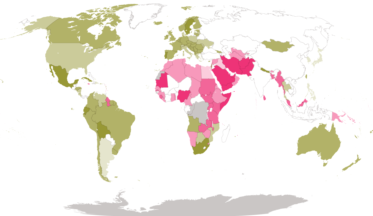
From a human rights perspective, it’s a lucky thing that “AI gaydar” doesn’t work so well, since as of 2022, homosexuality remains a criminal offense in 67 countries. In a number of them (Iran, Saudi Arabia, Yemen, Afghanistan, Brunei, Mauritania, Pakistan, Qatar, the United Arab Emirates, Nigeria, Uganda, and Somalia), it may be punishable by execution. Hence, in these countries, an accurate “gaydar camera” (together with the kind of ubiquitous surveillance increasingly common in public spaces) would amount to a dragnet technology for rounding up gay people, who are by definition “criminals,” for mass incarceration—or worse.
Remember that homosexuality was also criminalized in most Western countries until very recently. In England, it was punishable by death under the Buggery Act of 1533, which codified “sodomy” as a “detestable and abominable vice.” The 1861 Offences against the Person Act reduced the punishment to life imprisonment, and remained in force until 1967.
Both Oscar Wilde and Alan Turing were convicted under this law. At the time of Turing’s trial in 1952, he was not only a computer science pioneer, but also a war hero, having secretly cracked the Nazis’ Enigma codes, saving untold numbers of Allied lives. 42 Turing was sentenced to so-called “chemical castration” (feminizing estrogen injections, like those David Reimer underwent) as an alternative to prison. Like Oscar Wilde, Turing died in his forties, possibly of suicide. The British government had done its best to ruin both of their lives. Queen Elizabeth only officially “pardoned” Turing in 2013, nearly 60 years after his death. Wilde was “pardoned” in 2017, along with 50,000 other gay men on the far side of the grave. 43
Subtle biases in image quality, expression, and grooming can be picked up on by humans, so these biases can also be detected by AI. While Wang and Kosinski acknowledge grooming and style, they believe that the chief differences between their composite images relate to face shape, arguing that gay men’s faces are more “feminine” (narrower jaws, longer noses, larger foreheads) while lesbian faces are more “masculine” (larger jaws, shorter noses, smaller foreheads). As with less facial hair on gay men and darker skin on straight men, they suggest that the mechanism is gender-atypical hormonal exposure during development. This echoes the widely discredited 19th century “sexual inversion” model of homosexuality, as illustrated by Krafft-Ebing’s “Count Sandor V” case study among many others.
More likely, though, the differences are a matter of shooting angle. A 2017 paper on the head poses heterosexual people tend to adopt when they take selfies for Tinder profiles is revealing. 44 In this study, women are shown to be about 50% likelier than men to shoot from above, while men are more than twice as likely as women to shoot from below.
Shooting from below will have the apparent effect of enlarging the chin, shortening the nose, and attenuating the smile. This view emphasizes dominance—or, maybe more benignly, an expectation that the viewer will be shorter. On the other hand, shooting from above simulates a more submissive posture, while also making the face look younger, the eyes bigger, the face thinner, and the jaw smaller—though again, this can also be interpreted as an expectation or desire 45 for a potential partner (the selfie’s intended audience, after all) to be taller. If you’re seeking a same-sex partner, the partner will tend on average to be of the same height, so one would expect the average shot to be neither from below nor from above, but straight on.


And this is just what we see. Heterosexual men on average shoot from below, heterosexual women from above, and gay men and lesbian women from closer to eye level. 46 Notice that when a face is photographed from below, the nostrils are prominent (as in the heterosexual male face), while higher shooting angles hide them (as in the heterosexual female face). A similar pattern can be seen in the eyebrows: shooting from above makes them form more of a V shape, but they get flatter, and eventually caret-shaped (^) as the camera is lowered. Shooting from below also makes the outer corners of the eyes seem to droop. In short, the changes in the average positions of facial landmarks match what you’d expect to see from differing selfie angles.
Let’s turn this observation on its head: might the human smile and frown have their origins in dominant (taller, looking downward) and submissive (shorter, looking upward) head poses? If so, these expressions may originally have evolved, at least in part, to mimic the way facial appearance varies based on height and posture. 47
Indeed, there’s strong evidence that smiling is the human version of the “bared teeth face” or “fear grin” in monkeys, associated with submission or appeasement. 48 Submissive postures also tend to involve crouching and making one’s body look small, while dominant postures involve looking big and towering over others, or at least using head angle to seem taller—hence expressions like “acting superior” or “looking down your nose at someone.” I find it suggestive, also, that arching one’s eyebrows (which shortens the forehead and changes the eyebrow shape) is associated with a superior attitude.
Whatever the reasons, when we look at human faces today—especially static, two-dimensional photos of strangers taken under uncontrolled conditions—there’s a degree of visual ambiguity between head pose, the shapes of facial features, and affect (i.e. smiling or frowning).
In the heterosexual context, this may also explain the stereotypically more feminine look of the average “nice” or “trustworthy” face, and the more masculine character of the average “mean” or “untrustworthy” face. As researchers put it in a 2004 paper, Facial Appearance, Gender, and Emotion Expression,
[A] high forehead, a square jaw, and thicker eyebrows have been linked to perceptions of dominance and are typical for men’s faces […], whereas a rounded baby face is both feminine and perceived as more approachable […] and warm […], aspects of an affiliative or nurturing orientation. This leads to the hypothesis that—regardless of gender—individuals who appear to be more affiliative are expected to show more happiness, and individuals who appear to be more dominant are seen as more anger prone. As cues to gender and cues to affiliation/dominance are highly confounded, this would lead to more women being expected to be happiness prone and more men to be anger prone. 49

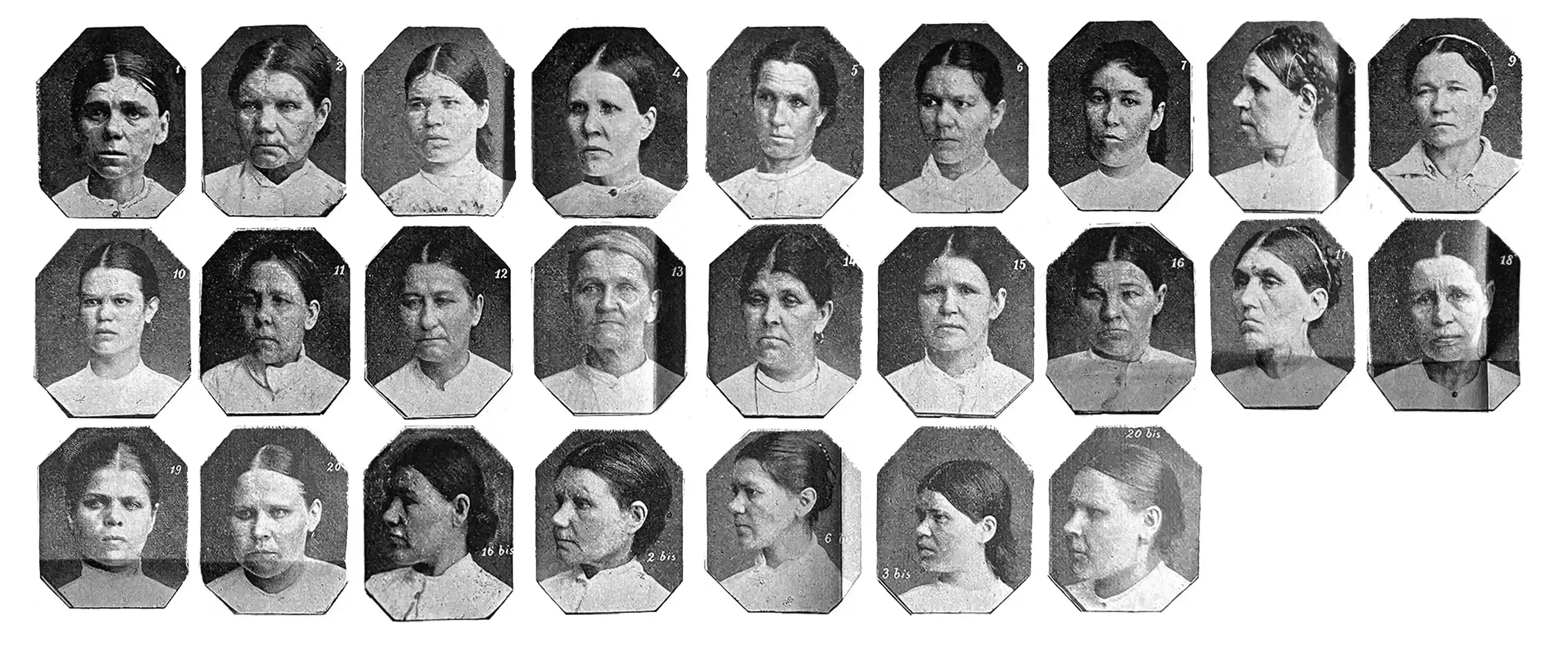
This brings us back once more to physiognomy. A woman with what appears to be an unsmiling, perhaps defiant expression, photographed in V.G. Rocine’s 1910 physiognomy primer Heads, Faces, Types, Races, supposedly illustrates “Degeneracy seen in [the] eyes, eyebrows, nose, lips, jaw, hair and pose.” 50 As with a collection of similar mugshots from Lombroso’s The criminal woman, a great majority of the female “crime” in question was either nonviolent and associated with poverty, or just reflected behavior that didn’t conform to prevailing gender and sexual norms. With so many biases in play, it’s hard to know which was judged first—women’s faces, or their actions.
Turing, “Computing Machinery and Intelligence,” 1950.
Hayles, How We Became Posthuman: Virtual Bodies in Cybernetics, Literature, and Informatics, xiii–xiv, 1999.
Keep in mind that the questions and patterns of responses are culturally specific. Long hair, for instance, has been and remains traditional for men in many cultures.
If you’re a math nerd, you may find this language imprecise… and that’s true. But I promised there would be no equations, and I’m bending that rule a little bit as it is in the next couple of paragraphs.
Calculating a PCA is a bit like long division from hell—it requires carrying out a complex, repetitive, many-step algorithm, which wasn’t practical to do before we had computers. If you’re interested in the mechanics, though, check out every old school data scientist’s must-have reference manual: William H. Press et al., Numerical Recipes 3rd Edition: The Art of Scientific Computing, 2007.
De Waal, Different: Gender Through the Eyes of a Primatologist, 51–52, 2022.
De Waal, 67.
And of course, in naming them, we would create a feedback loop: with our penchant for anonymous identities, many of us would modify our behavior to fall more clearly into one peak or the other, which would in turn influence our use of language. This describes, in short, how gender is constructed socially, albeit not beginning with a blank slate.
Chapter 12 points out the ways in which other cultures have variously defined a “third gender”; it’s possible that in certain cultural contexts, and given the right set of questions, a distinct cluster would emerge.
Imperva, “2022 Bad Bot Report,” 2022; Ikeda, “Bad Bot Traffic Report: Almost Half of All 2021 Internet Traffic Was Not Human,” 2022.
Turk and Pentland, “Eigenfaces for Recognition,” 1991.
Mike, “The Face of Tomorrow —the Human Face of Globalization,” 2004.
There are a few technicalities. For example: the hypothetical Stepford data are arranged so that all responses average to zero over the population. If they didn’t, the average response values would need to be subtracted out before calculating weights. (I did so for the handedness and gender presentation analyses.) Similarly, one would need to subtract from a selective facial composite the overall average face to produce the kind of optimal linear estimator described. Then, calculating an estimate involves multiplying the resulting pixel weights by the difference between an unknown portrait’s pixels and the average face.
Galton, “Composite Portraits,” 1878.
Agüera y Arcas, Mitchell, and Todorov, “Physiognomy’s New Clothes,” 2017.
Turk and Pentland, “Eigenfaces for Recognition,” 1991.
“The goal of the FERET program was to develop automatic face recognition capabilities that could be employed to assist security, intelligence, and law enforcement.” “Face Recognition Technology (FERET),” 2017.
Reichert, “Clearview AI Facial Recognition Customers Reportedly Include DOJ, FBI, ICE, Macy’s,” 2020.
Kushwaha et al., “Disguised Faces in the Wild,” 2018.
Harwell, “Facial Recognition Firm Clearview AI Tells Investors It’s Seeking Massive Expansion Beyond Law Enforcement,” 2022.
Snowden, Permanent Record, 2019.
Wu and Zhang, “Automated Inference on Criminality Using Face Images,” 2016; Wu and Zhang, “Responses to Critiques on Machine Learning of Criminality Perceptions (Addendum of arXiv:1611.04135),” 2017.
Many facial recognition engines exhibit racial bias. Most commonly, this takes the form of worse recognition performance for minorities underrepresented in the training data. Grother, Ngan, and Hanaoka, “Face Recognition Vendor Test Part 3: Demographic Effects,” 2019.
Cogsdill et al., “Inferring Character from Faces: A Developmental Study,” 2014.
Oosterhof and Todorov, “The Functional Basis of Face Evaluation,” 2008.
Peterson et al., “Deep Models of Superficial Face Judgments,” 2022.
Olivola, Funk, and Todorov, “Social Attributions from Faces Bias Human Choices,” 2014.
Todorov et al., “Social Attributions from Faces: Determinants, Consequences, Accuracy, and Functional Significance,” 2015.
Holtz, “From First Impression to Fairness Perception: Investigating the Impact of Initial Trustworthiness Beliefs,” 2015.
Rezlescu et al., “Unfakeable Facial Configurations Affect Strategic Choices in Trust Games With or Without Information About Past Behavior,” 2012.
Wilson and Rule, “Facial Trustworthiness Predicts Extreme Criminal-Sentencing Outcomes,” 2015.
Efferson and Vogt, “Viewing Men’s Faces Does Not Lead to Accurate Predictions of Trustworthiness,” 2013.
Wang and Kosinski, “Deep Neural Networks Are More Accurate than Humans at Detecting Sexual Orientation from Facial Images,” 2018.
“Advances in AI Are Used to Spot Signs of Sexuality,” 2017.
Anderson, “GLAAD and HRC Call on Stanford University & Responsible Media to Debunk Dangerous & Flawed Report Claiming to Identify LGBTQ People Through Facial Recognition Technology,” 2017.
Levin, “Face-Reading AI Will Be Able to Detect Your Politics and IQ, Professor Says,” 2017.
Clearly this is an incomplete accounting of sexual orientations, as well as presuming a gender binary. The problems inherent in AI systems that make such discrete classifications of people are well described in Katyal and Jung, “The Gender Panopticon: AI, Gender, and Design Justice,” 2021.
Margaret Mitchell is an AI researcher, and Alex Todorov is a world expert on the social perception of faces. Todorov co-authored several papers cited in this chapter, and has published a book on the topic: Todorov, Face Value: The Irresistible Influence of First Impressions, 2017. I also went back on the Savage Lovecast to talk about this work in November of 2017; see Savage, “Episode #579,” 2017.
These figures rise to 91% for men and 83% for women if 5 images are considered.
Cox et al., “Inferences About Sexual Orientation: The Roles of Stereotypes, Faces, and the Gaydar Myth,” 2016.
Rule and Ambady, “Brief Exposures: Male Sexual Orientation Is Accurately Perceived at 50ms,” 2008.
Estimates range from 2 to more than 20 million lives. Drury, “Alan Turing: The Father of Modern Computing Credited with Saving Millions of Lives,” 2019; Copeland, “Alan Turing: The Codebreaker Who Saved ‘Millions of Lives,’” 2012.
McCann, “Turing’s Law: Oscar Wilde Among 50,000 Convicted Gay Men Granted Posthumous Pardons,” 2017.
Sedgewick, Flath, and Elias, “Presenting Your Best Self(ie): The Influence of Gender on Vertical Orientation of Selfies on Tinder,” 2017.
Per Fink et al., “Variable Preferences for Sexual Dimorphism in Stature (SDS): Further Evidence for an Adjustment in Relation to Own Height,” 2007.: “[…] evidence suggests that females prefer taller over shorter males, indeed taller males have been found to have greater reproductive success […] relative height is also important […] people adjust their preferences […] in relation to their own height in order to increase their potential pool of partners.” The finding held in all three countries studied—Austria, Germany, and the UK—as well as in an earlier Polish study.
Although the authors use a face recognition engine designed to try to cancel out effects of head pose and expression, my research group confirmed experimentally that this doesn’t work, a finding replicated by Tom White, a researcher at Victoria University in New Zealand. White, “I expected a ‘face angle’ classifier using vggface features would perform well, but was still floored by 100% accuracy over 576 test images,” 2017.
Parr and Waller, “Understanding Chimpanzee Facial Expression: Insights into the Evolution of Communication,” 2006.
Dunbar, Friends, 186, 2021.
Hess, Adams, and Kleck, “Facial Appearance, Gender, and Emotion Expression,” 2004.
Rocine, 171.